![[attach.png]](idldoc-resources/xattach.png.pagespeed.ic.tvtntcUO-o.png)
./
pp_convol.pro
Author information
- Author
Paulo Penteado (pp.penteado@gmail.com), Feb/2010
Routines
Routines from pp_convol.pro
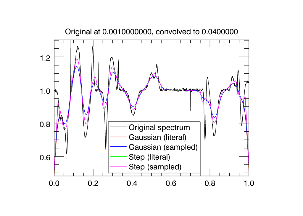
pp_convol_test [, width]Examples to test and illustrate the different behaviors of pp_convol.
result = pp_convol(y, x [, step=step] [, gaussian=gaussian], width=width [, grid_tolerance=grid_tolerance] [, kernelx=kernelx] [, kernely=kernely] [, local=local] [, newton=newton] [, lsquadratic=lsquadratic] [, quadratic=quadratic] [, spline=spline] [, xinc=xinc] [, yinc=yinc] [, xstart=xstart] [, xend=xend] [, xbox=xbox] [, ybox=ybox])Convolves the provided y(x) function with either a rectangular or Gaussian kernel of the given width, or the provided arbitrary kernel (not yet implemented).
Routine details
top source pp_convol_test
pp_convol_test [, width]
Examples to test and illustrate the different behaviors of pp_convol.
Makes up a high resolution spectrum and convolves it to lower resolutions.
Parameters
- width in optional default=0.04
The width for the convolution kernels.
Examples
Convolve spectra to different resolutions:
 .com pp_convol ;pp_convol_test is in pp_convol.pro, so it will not be found by itself
 pp_convol_test,0.04
 pp_convol_test,0.02

Author information
- Author:
Paulo Penteado (pp.penteado@gmail.com), Feb/2010
Other attributes
- Uses:
Statistics
| Lines: | 25 lines |
| Cyclomatic complexity: | 2 |
| Modified cyclomatic complexity: | 2 |
top source pp_convol
result = pp_convol(y, x [, step=step] [, gaussian=gaussian], width=width [, grid_tolerance=grid_tolerance] [, kernelx=kernelx] [, kernely=kernely] [, local=local] [, newton=newton] [, lsquadratic=lsquadratic] [, quadratic=quadratic] [, spline=spline] [, xinc=xinc] [, yinc=yinc] [, xstart=xstart] [, xend=xend] [, xbox=xbox] [, ybox=ybox])
Convolves the provided y(x) function with either a rectangular or Gaussian kernel of the given width, or the provided arbitrary kernel (not yet implemented).
The x grid does not need to be regular, and, contrary to common practice, no resampling is done to a regular grid to calculate the convolution (resampling is not needed). Also contrary to common practice, for rectangular or Gaussian kernels the integral is done analytically, not numerically. In the case of a Gaussian kernel, it extends from the Gaussian center up to the point where the terms in the integral become 0 (at double precision).
Also, this routine allows for both literal and sampled interpretations of the input function (set with the local keyword).
Return value
The result of the convultion is given for the same x locations as the input, there is no automatic resampling. If resampling is intended after the convolution, pp_resampled is recommended, as it preserves the areas.
Parameters
- y in required
An array with the function values corresponding to the locations in x.
- x in required
An array of locations where the function is sampled. Must be ordered (increasing or decreasing).
Keywords
- step in optional default=1
If set, the convolution kernel is a rectangular function of the given width.
- gaussian in optional default=0
If set, the convolution kernel is a Gaussian, of fwhm of the given width.
- width in required
The width of the convolution kernel (for step or gaussian).
- grid_tolerance in optional default=1d-6
Not yet implemented. Specifies the maximum fractional variation in the input grid to accept it as uniform.
If the input grid is found to be uniform, the integration can be done faster.
- kernelx in optional
Not yet implemented. An array of the x locations (centered at x=0) of the arbitrary convolution kernel to use.
Must be ordered in increasing x.
- kernely in optional
Not yet implemented. An array of the the arbitrary convolution kernel's values to use. Must make a function of unit area.
- local in optional default=0
If not set, the y values are interpreted as a measured sample, that is, as the average of the "flux" falling inside the region centered at the corresponding x values: x locations are interpreted as the centers of bins. Since this interpretation is equivalent to a literal interpretation of a function made of rectangular regions, in this method there are no interpolations (partial areas, if any, are just the corresponding fractions of the rectangles).
If set, interprets the input function literally.
- newton in optional default=0
Passed on to pp_integral. If local is set and newton is set, the function integrations are done with int_tabulated, which uses a 5 point Newton-Cotes formula. If local is not set, this has no effect.
- lsquadratic in optional default=0
Passed on to pp_integral. If the method requires interpolation, this is passed on to interpol, to select 4 point quadratic interpolation.
If none of lsquadratic, quadratic and spline are set, interpolation is linear.
- quadratic in optional default=0
Passed on to pp_integral. If the method requires interpolation, this is passed on to interpol, to select 3 point quadratic interpolation.
If none of lsquadratic, quadratic and spline are set, interpolation is linear.
- spline in optional default=0
Passed on to pp_integral. If the method requires interpolation, this is passed on to interpol, to select spline interpolation.
If none of lsquadratic, quadratic and spline are set, interpolation is linear.
- xinc out optional
Returns the x values, in increasing order.
- yinc out optional
Returns the y values, in order of increasing x.
- xstart out optional
If local is not set, returns the location where each input pixel starts. If local is set, this is ignored.
- xend out optional
If local is not set, returns the location where each input pixel ends. If local is set, this is ignored.
- xbox out optional
Used when not in local mode, to return the input x values in pairs of equal values, so that plotting xbox,ybox shows the rectangles that are how the input values were interpreted.
- ybox out optional
Used when not in local mode, to return the input y values in pairs of equal values, so that plotting xbox,ybox shows the rectangles that are how the input values were interpreted.
Examples
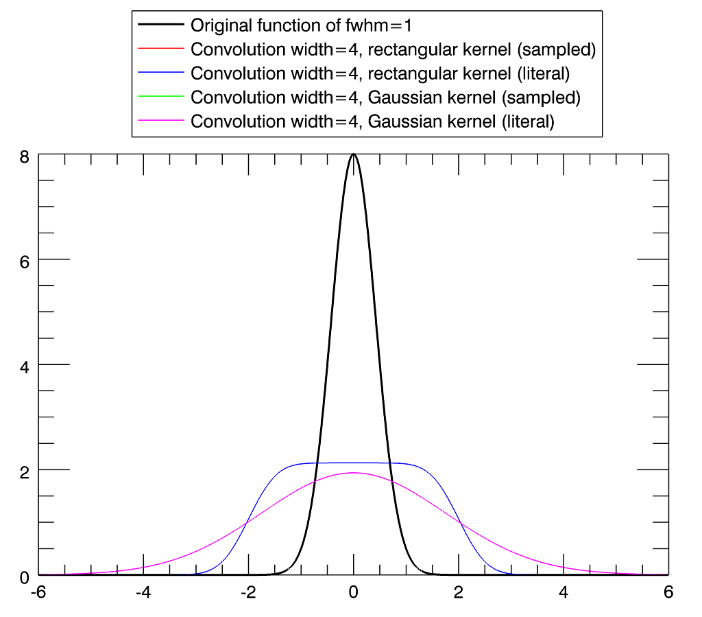
Make a well-sampled input function y(x) with fwhm=1:
 x=(12d0*dindgen(1001)/1d3)-6d0
 y=exp(-(x^2*4d0*alog(2d0)))*8d0
 iplot,x,y,/isotropic,name='Original function of fwhm=1',/insert_legend,thick=2.
 yc1=pp_convol(y,x,/step,width=4d0)
 iplot,x,yc1,/over,color=[255,0,0],name='Convolution width=4, rectangular kernel (sampled)',/insert_legend
 yc2=pp_convol(y,x,/step,/local,width=4d0)
 iplot,x,yc2,/over,color=[0,0,255],name='Convolution width=4, rectangular kernel (literal)',/insert_legend
 yc3=pp_convol(y,x,/gaussian,width=4d0)
 iplot,x,yc3,/over,color=[0,255,0],name='Convolution width=4, Gaussian kernel (sampled)',/insert_legend
 yc4=pp_convol(y,x,/gaussian,width=4d0,/local)
 iplot,x,yc4,/over,color=[255,0,255],name='Convolution width=4, Gaussian kernel (literal)',/insert_legend
See also the example in pp_convol_test, for a comparison of the methods with a more realistic (spectrum-like) function.
Author information
- Author:
Paulo Penteado (pp.penteado@gmail.com), Feb/2010
Other attributes
- Todo:
Implement arbitrary kernel, grid_tolerance, and quadratic and cubic Gaussian integrations.
- Uses:
Statistics
| Lines: | 101 lines |
| Cyclomatic complexity: | 17 |
| Modified cyclomatic complexity: | 17 |
File attributes
| Modification date: | Wed Jun 29 22:15:28 2016 |
| Lines: | 126 |
| Docformat: | rst rst |